Risk Assessment
CPM User's Guide
CPM Conversion
Welcome to the EPA Superfund "Counts Per Minute (CPM) Calculator" user's guide. Here, you will find instructions on how to use the calculator and supporting technical documentation explaining the conversion to cpm process. Additional guidance is also provided on the limitations and intended use of this calculator. It is suggested that users read the CPM FAQ page before proceeding. The user guide is extensive, so please use the "Open All Sections" and "Close All Sections" links below as needed. Individual sections can be opened and closed by clicking on the section titles. Before proceeding through the user's guide, please read the Disclaimer. In addition, Users of the CPM at a CERCLA site should consult with EPA Headquarters, Stuart Walker at Walker.Stuart@epa.gov (202-566-1148), David Kappelman at Kappelman.David@epa.gov (513-487-6540), and Jack Burn at Burn.James@epa.gov (334-270-3437).
Open All Sections | Close All Sections
Disclaimer
This guidance document sets forth EPA's recommended approaches based upon currently available information for estimating detector readings that correspond to remedial criteria at Comprehensive Environmental Response, Compensation, and Liability Act (CERCLA) sites (commonly known as Superfund). This document does not establish binding rules. Alternative approaches for estimating detector readings may be more appropriate at specific sites (e.g., where site circumstances do not match the underlying assumptions, conditions, and models of this guidance). The decision whether to use an alternative approach and a description of any such approach should be documented. Accordingly, when comments are received at individual sites questioning the use of the approaches recommended in this guidance, the comments should be considered and an explanation provided for the selected approach.
The policies set out in the CPM User's Guide provide guidance to EPA staff. It also provides guidance to the public and regulated community on how EPA intends to estimate detector readings. EPA may change this guidance in the future, as appropriate.
It should also be noted that estimating detector readings is not intended to replace sampling. Verification samples will still be necessary to appropriately conduct radiation surveys. Use of the CPM output is intended to reduce the number of laboratory samples and not eliminate them. The CPM Calculator has many limitations that are detailed in the user's guide.
This web calculator may be used to estimate detector readings for radionuclides in several different media. The calculator is flexible and may be used to derive site-specific detector readings as more site characterization is obtained. This is particularly true if the contamination source depth from surface varies.
1. Introduction
Field sampling is a necessary step of environmental remediation. Field sampling establishes areas of contamination before, during, and after site characterization in order to ensure only acceptable residual levels of contamination remain. Sampling has the potential to be an extremely time-consuming and costly portion of a radiological site remediation. Collected samples must be shipped to an off-site laboratory or counted in an on-site mobile unit in order to establish areas of contamination and to ensure that remaining contaminants are of acceptable residual levels. This tool calculates the radiation detector reading in counts per minute (cpm) that corresponds to the level of radioactivity in a surface or volume of medium by converting radioactivity from either pCi/cm2 or pCi/g to cpm
The CPM Calculator is a web-based calculator that estimates a photon detector response for a target level of contamination in a source medium. This calculator can be used to determine screening levels in cpm that are based on pCi per volume or area. Using handheld detectors, measuring cpm can help reduce costly laboratory sampling. A correction factor for cpm analysis established between this calculator's results and lab sampling analysis may be needed to account for ground truthing and other field nuances like roughness factors.
The user should always verify CPM Calculator results with lab sampling.
Features of the CPM Calculator include:
- option to calculate the Gross Detector Response (GDR) for a single radionuclide or multiple radionuclide mixtures according to MARSSIM guidance,
- option to include progeny presence,
- choice of target activity concentration,
- truncated decay chains, which allow for man-made radonuclide decay spectrum,
- choice between 4 cylindrical NaI scintillation detector configurations (0.5" × 1", 1" × 1", 2" × 2", and 3" × 3"),
- choice of 7 contamination depths (ground plane, 1 cm, 2 cm, 3 cm, 5 cm, 15 cm, and infinite depth), and
- choice of 6 source materials (soil, steel, concrete, glass, wood, and drywall).
2. Understanding the CPM Calculator
This section presents a general overview of the CPM Calculator. See section 4 for greater detail.
2.1 General Considerations
The gross detector response (GDR) is produced by the CPM calculator for the isotopes and activity concentrations selected to represent the site. The GDR is estimated from Monte Carlo (MC) radiation transport code simulations that were used to derive a conversion factor (CF) representative of the source radionuclide(s), contaminated media type, detector size, distance from the source, and depth of source contamination from the surface. With multiple variables, limitations of the tool are expected.
2.2 Limitations of the CPM Calculator
Limitations of the GDR calculations are discussed here. It is expected that a correction factor will need to be derived based on differences between the theoretical GDR value from the CPM Calculator and the site measured GDR.
2.2.1 The Model
The CPM Calculator model was developed using MC to simulate the spectrum of desired radionuclide(s). The CPM Calculator does not replace lab-based sampling or MARSSIM final status survey requirements; however, it may provide a reasonable starting point from which to work. A correction factor for cpm analysis, established between this calculator's results and lab sampling analysis, should be applied to account for site-specific factors that depart from the idealized simulations, such as ground truthing and other field nuances.
In the MC modeling, it is important to note that only the distribution of energy deposition pulses in the detector crystals are simulated; therefore, other factors that comprise the true detector response such as detector resolution, dead time, background, and pulse pile-up are unaccounted for.
2.2.2 Uniformity
The model assumes uniform contamination on the source surface or in chosen media volume. In other words, the radionuclides of interest are in constant ratio to each other, and the source is infinite in lateral extent. Incongruity of the radionuclide ratios, such as separate spills or cross-contaminated sites, will diminish the effectiveness of the CPM calculator. In addition to the CPM results being applicable to homogenous sites, the FACs can vary across the site and representative activities should be entered into the calculator.
The assumed soil composition is typical of silty soil (Veinot, 2017) containing 30 percent water and 20 percent air by volume. The assumed soil density is 1.6 × 10³ kg m3.
2.2.3 Photon Emitters
Radionuclides that emit alpha and beta radiation are difficult to measure with any accuracy in the field and are omitted from this model, unless the radionuclide also emits a qualifying photon.
A qualifying photon is one with energy between 20 keV and 3 MeV and with a decay yield greater than 0.1%. The energy cutoff is due to the energy response curve in the model detector manufacturer's specifications. For more information, see the FAQ page.
Bremsstrahlung radiation is electromagnetic radiation produced by the deceleration of a charged particle when deflected by another charged particle, typically an electron deflected by an atomic nucleus. The moving particle loses kinetic energy and is then converted into a photon. A study of radiation contribution from primary source electrons emitted from the modeled materials is under consideration.
2.2.4 Background Radiation
The model does not account for background radiation. The user is responsible for adding or subtracting any background counts to or from the GDR.
2.2.5 Shielding
The model does not account for any shielding that may be present above the source. Examples of shielding may include water and grass.
2.2.6 Low GDR Results
Calculator output of the GDR may be lower than some detectors can resolve when the desired TACs are near background. The CPM results may be less than instrument detection limits, critical values, or within instrument counting uncertainty. When such results are given by the calculator, their applicability may be lost. Consider using background counts as an indication of nearing remediation completion.
2.3 CPM Output
See section 3 for detailed information on running the calculator and interpreting the output.
2.4 Radionuclide-Specific Parameters
Several radionuclide-specific parameters are needed for development of the GDRs. The parameter sources are identified here.
2.5 CPM results in the Context of Superfund Modeling Framework
This CPM calculator focuses on the estimation of detector readings that may be used as part of the larger framework to determine if a site complies with remediation criteria. Criteria that can be converted to cpm in this tool can come from the PRG, BPRG, SPRG, DCC, BDCC, and SDCC Calculators or concentrations in ARARs. The user's guides for these calculators should be consulted prior to entering their results as Target Activity Concentrations in the CPM Calculator.
Prior to using another model for GDR at a CERCLA remedial site, EPA regional staff should consult with the Superfund remedial program's National Radiation Expert (Stuart Walker, (202)-566-1148, walker.stuart@epa.gov).
3. Using the CPM Website
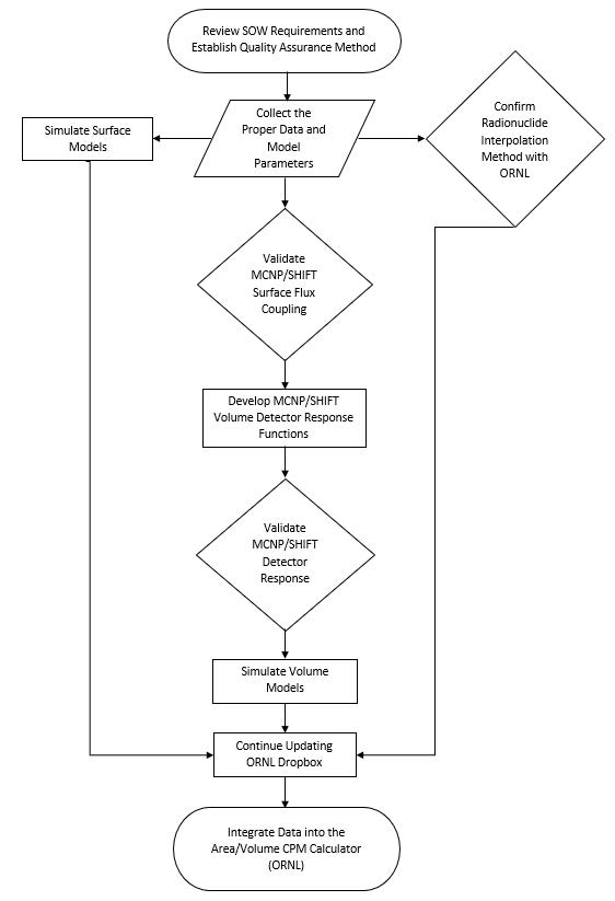
This section provides a step-by-step guide for each page of the CPM calculator and highlights potential issues that may be encountered.

This Flow Chart presents the general logic flow of the CPM calculator for each decay method. Click here for full-size image.
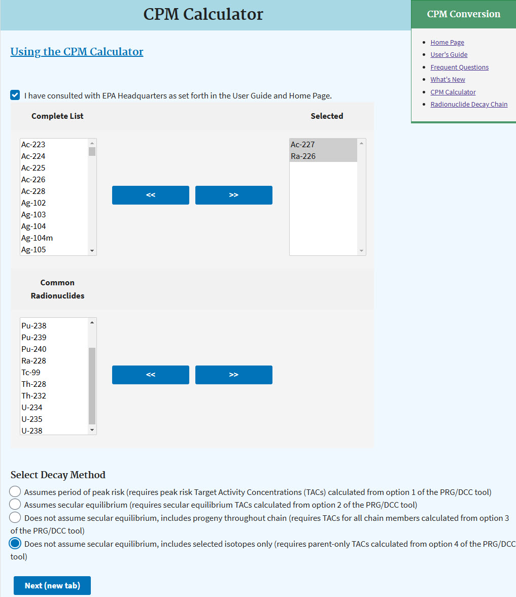
3.1 Selecting Radionuclides of Interest
There are two picklists to choose from. The first picklist, "Complete List", includes all radionuclides that are available. The second picklist, "Common Radionuclides", includes common radionuclides, many of which are found at Superfund sites. To select a radionuclide, click on its name to highlight the selection. Next, click the blue button with arrows to move that radionuclide to the Selected box. Multiple radionuclides can be moved together by holding the shift or control keys while clicking on radionuclide names. To remove a radionuclide from the "Selected" box, highlight it and click the blue button with the arrows pointing back to the box from which it came.
After selecting radionuclides, select the decay method that was used to calculate the TAC(s). Chains with very long-lived progeny have been truncated at the typical 'parent' radionuclides for man- made purposes.
The following 14 radionuclides are included in the Common Radionuclides list: Am-241, Co-60, Cs-137, Pu-238, Pu-239, Pu-240, Ra-226, Ra-228, Tc-99, Th-228, Th- 232, U-234, U-235, and U-238.
Before leaving the page, you need to verifiy in a check box that you have read the user's guide and FAQ to grasp the limitations and intended use of the calculator.
When all the desired radionuclides have been selected, click "Next (new tab)".
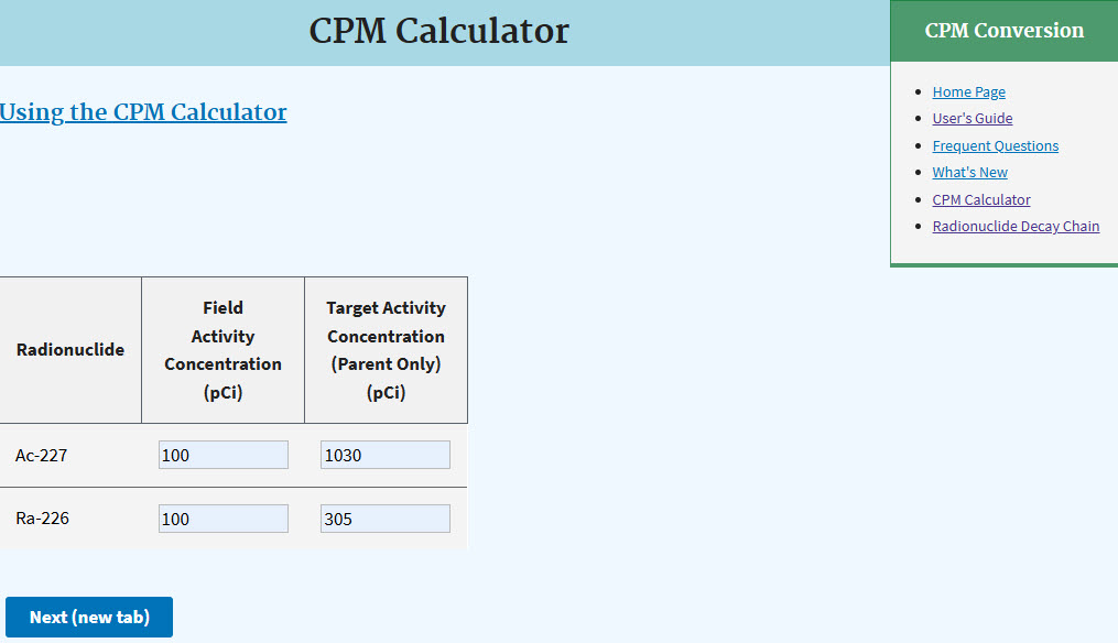
3.2 Target and Field Activity Concentrations
Enter the target activity concentrations (TAC) in pCi/cm2 or pCi/g for each radionuclide. Do not mix units. The TAC is the activity for which the result in cpm is desired. The TAC may be concentrations specified in an ARAR or concentrations developed using the following EPA Calculators:
- the PRG Calculator for radionuclide cancer risk for soil,
- the DCC Calculator to assess radionuclide dose for soil,
- the BPRG Calculator for radionuclide cancer risk inside buildings,
- the BDCC Calculator for radionuclide dose inside buildings,
- the SPRG Calculator to assess radionuclide cancer risk for hard outside surfaces, and
- the SDCC Calculator for radionuclide dose for hard outside surfaces.
If multiple radionuclides are selected, enter the field activity concentration (FAC) for each radionuclide. The FAC, which is based on laboratory analysis, is the activity of each primary radionuclide in the contaminated source and is used to find the radionuclide ratios in mixtures. The FACs are used to find the relative fractions of each radionuclide, which are then applied to the GDR. Click "Next (new tab)".
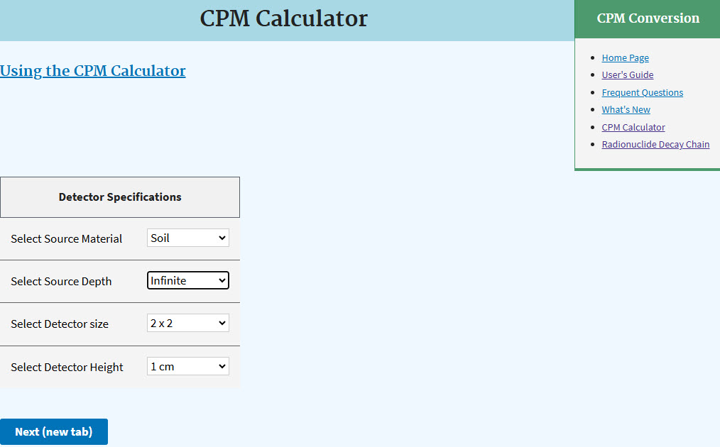
3.3 Detector and Material Information
On this page, the details of the detector used and the details of contaminated media are required.
- Select the source material of interest.
- Select the uniform depth of contamination in the source material.
- Select the scintillation detector size.
- Select the detector height above the source.
- Click "Next (new tab)".
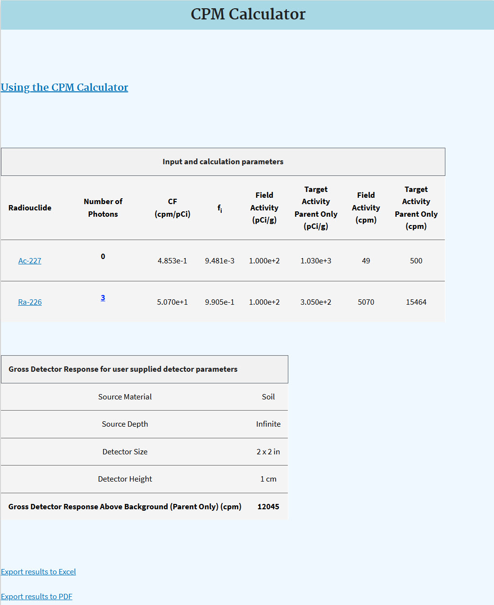
3.4 Results - Gross Detector Response
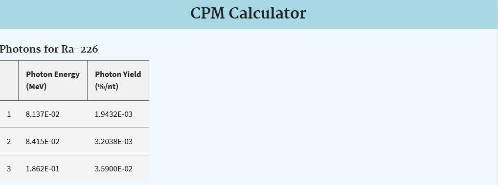
On this page, the GDR approximates meeting the TAC for the radionuclides selected. The inputs for source material, source depth, detector size, and detector height are repeated. Additionally, the photon energy and yield are presented on a new page, if one clicks on the highlighted numbers in the Number of Photons column. If any photon energies are out of the range of the detector, they are identified on this page with an asterisk.
4. Technical Documentation
This section presents the details of the GDR calculation process.
4.1 Overview of Design
This section describes the methods for the surface and volumetric calculations used in the CPM calculator. The Monte Carlo N-Particle (MCNP) v6.2 radiation transport code was utilized to model the CPM calculator surface contamination by simulating the average energy deposition pulse height tally (Werner (ed.), 2017). A detector response function methodology (Asano et al., 2022), combining capabilities in MCNP with hybrid radiation transport capabilities implemented in the MC code Shift (Pandaya et al., 2016), was used to derive the Volume CPM CFs in a computationally feasible manner. The latter methodology is herein referred to as the "MCNP/Shift method". Since Shift currently does not support a pulse height tally, the average cell flux in Shift was used to approximate the MCNP-equivalent pulse height for cases involving buried source attenuation. Previous benchmarking of Shift capabilities indicated that radiation transport of photons through contaminated volumetric depths, as required in the volume CPM function, superseded capabilities of MCNP in default mode by a speed factor of 10 for simulations of average cell flux. The ability to conduct rapid, high-fidelity radiation transport simulations was paramount for this initiative, given the initially desired 23,120 discrete simulations for a series of contamination depths, 19 monoenergetic photon energies, 17 photon emitting radionuclides, and four NaI(Tl) scintillation detector models outlined in the table shown below. The small amount of thallium doping material in the detector crystals was omitted in the MCNP and Shift models for simplicity; this has a negligible effect on the energy deposition-based GDR, since the total mass attenuation coefficient is largely dependent on the sodium and iodide material concentrations.
Material Monoenergetic Energies Radionuclide Energies Contamination Depths Detector Distances Number of Detectors Total Runs Concrete 19 17 7 5 4 5,320 Drywall 19 17 4 5 4 3,040 Glass 19 17 4 5 4 3,040 Soil 19 17 7 5 4 5,320 Steel 19 17 7 5 4 5,320 Wood 19 17 5 5 4 3,800 Total 23,120 Parameters modeled and simulated in MCNP and Shift included the following: plane radii, discrete photon energies, Superfund radionuclides (Am- 241, Co-60, Ba-137m/Cs-137, Pu-238, Pu-239, Pu-240, Ra-226, Ra-228, Tc-99, Th-228, Th-230, Th-232, U-234, U-235, U-238/Pa-234m), and source material compositions. All Four NaI(Tl) scintillation detectors (0.5" × 1", 1" × 1", 2" × 2", 3" × 3") and source-detector distances of 0.5 cm, 1 cm, 2.54 cm, 10 cm, 30 cm were modeled. Contaminated media of soil, concrete, wood, steel, drywall, and glass were evaluated for depths (source thicknesses) of ground plane (surface), 1 cm, 2 cm, 3 cm, 5 cm, 15 cm, and infinite. Nineteen discrete energies between 20 keV and 3 MeV were evaluated (0.02, 0.03, 0.04, 0.05, 0.06, 0.07, 0.08, 0.1, 0.15, 0.2, 0.3, 0.4, 0.5, 0.6, 0.8, 1.0, 1.5, 2.0, and 3.0 MeV). Additionally, the list of radionuclides has been extended to include all radionuclides from ICRP 107 that satisfy the photon emission criteria previously described. Notably, both Rn-220 and Rn-222 lack the criteria for photon emission and have therefore been eliminated. In order to eliminate the computational runtime of simulating the photon emitting radionuclide spectra in MCNP or Shift, an interpolation method was employed to approximate the radionuclide CFs.
The table below presents the source thicknesses that were initially considered for each media. For some material and discrete energy combinations, the infinite thickness may be less than the discrete thickness value considered. Hence, for cases where the discrete simulation thickness is greater than four mean free paths, the source depth was not evaluated. Over the four detector sizes evaluated, 156 of the 23,120 possible combinations were not evaluated.
Material Ground Plane 1cm 2cm 3cm 5cm 15cm Infinite Soil Yes Yes Yes Yes Yes Yes Yes Concrete Yes Yes Yes Yes Yes Yes Yes Wood Yes Yes Yes Yes Yes No No Steel Yes Yes Yes Yes Yes Yes No Glass Yes Yes Yes Yes No No No Drywall Yes Yes Yes Yes No No No Only primary photon source emissions were considered, due to Shift's capability to conduct neutral particle and not charged particle transport. Therefore, beta emissions from the radionuclide of interest as well as pure beta-emitters (H-3 and Sr-90) and their associated bremsstrahlung emissions cannot be run using Shift and were therefore not addressed. A flow chart is provided below to summarize the approach.
4.2 Design Testing and Benchmarking
Both MCNP and SHIFT software packages were considered for the CPM Calculator design. Each was tested and benchmarked against the other for repeatability and speed.
MCNP is a stochastic method that is widely used to solve radiation transport problems in reactor physics, shielding, dosimetry, radiation detection and measurements, and various other applications of interest. The Monte Carlo (MC) method enables detailed, explicit geometric, energy, and angular representations and hence is considered the most accurate method available for solving complex radiation transport problems (Wagner et al., 2011). MCNP functions by simulating the individual average particle behavior in a given environment based on sampling the probability density of particles in phase space. The "behavior" of a particle may be described by the types of interactions (neutron capture, photon scatter, photon leakage, etc.) or "events" that are sampled from probability distributions containing transport data based on the selection of a pseudorandom number. In MCNP, the lifetime of an individual particle from birth until termination (due to absorption, escape from the problem boundary) is described as its random "history."
At the end of the simulation, the final average quantities of interest, known as tallies (such as flux, detector pulse, dose, etc.), are estimated from the distribution of all histories and have an associated uncertainty (relative error) that is proportional to one over the square root of the total number of histories for statistically well-behaved simulations. Therefore, the uncertainty may be decreased by increasing the number of histories simulated in the problem to coincide with the "law of large numbers," where the sample mean approaches the population mean as the sample size increases. While MCNP is considered to be the most accurate method available for solving complex radiation transport problems, it possesses the inherent disadvantage of being computationally expensive, as the required number of histories to reach proper convergence (less than 5% for detector pulse height) is increased for complex problems (LANL, 2003).
SHIFT is a massively parallel Monte Carlo radiation transport package that implements hybrid methods (deterministic coupled with stochastic) to obtain a faster and more accurate solution to problems of interest, as opposed to purely stochastic Monte Carlo. The hybrid methodology utilized in this study is known as the CADIS (Consistent Adjoint Driven Importance Sampling) method, which is a tally optimization method that relies on the discrete ordinates deterministic solver, Denovo, as part of the Exnihilo code suite to generate an adjoint flux and associated importance map for particles simulated in a given environment. Once the adjoint flux and importance map is generated, particles are more likely to be born in regions of higher importance in the simulation environment. The CADIS method is known to be 10-100,000 times more efficient than analog (no variance reduction) Monte Carlo based on tally figure of merit (FOM) comparisons (Biondo et al., 2017). The hybrid capabilities of SHIFT are particularly useful for speeding up the transport of sources that undergo significant attenuation in large problem geometries as well as lowering the variance of tally results when compared to analog Monte Carlo. SHIFT is currently capable of neutral particle transport for only photons and neutrons and may be used to simulate select tallies that mirror those included in MCNP, such as average flux in a volumetric cell (F4 in MCNP).
A benchmark of SHIFT capabilities indicated that radiation transport of photons through contaminated volumetric depths, as required in the Volume CPM function, supersedes capabilities of MCNP by a speed factor of 10 for simulations of track length estimate of cell flux. The ability to conduct rapid, high-fidelity radiation transport simulations is paramount for this initiative, for 23,120 discrete simulations for a series of contamination depths, 19 monoenergetic photon energies, 17 photon emitting radionuclides, and four NaI(Tl) detector models, summarized Table 3. Photon emitters were alone considered from the list due to SHIFT's capability to conduct neutral particle and not charged particle transport. Any primary or secondary charged particle transport requires the use of Monte Carlo code (e.g., MCNP). Therefore, beta emissions from the list of radionuclides as well as pure beta- emitters (H-3 and Sr-90) and their associated radiative components cannot be run using SHIFT. In addition, both Rn-220 and Rn-222 lack the criteria for photon emission and have also been eliminated as photon emitters. These criteria reduce the list of Superfund Common Radionuclides to the photon emitting radionuclides.
Note that Bremsstrahlung beta (+/-) particle transport and annihilations from positron emissions, for the listed radionuclides, were not considered. Should photons from these actions be expected, further analysis would be necessary to accurately predict the GDR.
4.2.1 Denovo Deterministic Solver Overview
A 3-D discrete ordinates transport solver utilized in Shift, known as Denovo, discretizes (conversion of continuous space to equivalent discrete space) the steady-state Boltzmann transport equation in space, angle, and energy to approximate the adjoint fluxes (importance functions that describe the expected tally contribution of particles) that are used to generate variance reduction parameters for accelerating fixed-source MC simulations (Wagner et al., 2011). The CPM Calculator photon sources are fixed, following the matrix equation:

as opposed to a k-eigenvalue sources, following the characteristic equation:

For brevity, all equations shown to demonstrate Shift's capabilities are derived. The steady-state Boltzmann transport equation solved in Denovo is given by (Evans et al., 2010):

Here, the state is defined by the angular flux ψ, and the independent variables are r = (x,y,z) (in centimeters); Ω = (θ,ψ) (in steradians); and E (in mega-electron-volts) representing space, angle, and energy, respectively (Evans et al., 2010). This equation may be used to describe how various particle types (i.e., neutrons, photons) travel through a medium. The variables on the left side of the above equation describe the net transport (leakage) and total interactions that the particle undergoes, respectively. The variables on the right side describe the total accumulated source density. The above equation is converted to a discrete angular form that accounts for anisotropic scattering of the source within a problem geometry (Evans et al., 2010), as shown here:

In simpler terms, the above equation represents the continuous steady-state Boltzmann transport equation in a discrete space, such that Denovo can solve for the flux component through discretization over the problem geometry "mesh" that is defined by the user with respect to space and angle. This equation accounts for group (g) scattering (with respect to energy and angle) as well as even and odd spherical harmonics functions (Ye,Yo) used to evaluate Legendre polynomials that expand the angular flux scattering cross section.
The above equation may be expressed in operator form (Evans et al., 2010):

The same principle applies, where "L" represents the differential transport operator describing the net transport and total interactions of the source (left-hand side of the above equations). The "M" operator is used to convert the harmonic moments to discrete angles; the "S" operator defines the group transfer cross sections for particles (scattering from one energy group to another): and qe represents the external source term (for photons this is negligible in the current study). The above equation may be further expanded to depict what Denovo is solving in matrix form (Evans et al., 2010):

The goal is to solve for the angular flux groups, given by [ψ]G. Shift couples SCALE continuous-energy (Shift MC solver) and multigroup physics (Shift MC solver and Denovo deterministic solver) cross section libraries for hybrid transport. The CPM Calculator photon sources discretized in Denovo are separable energy-space isotropic sources, which facilitate the hybrid methods. As opposed to traditional (Sn) iterative discretization methods, Denovo utilizes the Koch-Baker-Alcouffe (KBA) parallel sweep algorithm to perform a 2-D decomposition of a 3-D cartesian orthogonal structured spatial mesh (i.e., the simulation problem space) to solve the steady-state Boltzmann transport equation in space, angle, and energy (Evans et al., 2010). In other words, the KBA algorithm directly inverts the "L" term in the matrix form to obtain a more computationally efficient solution of the angular flux by "sweeping" through the 3-D cartesian orthogonal structured spatial mesh, as opposed to traditional source iteration techniques that may take longer converge. The defined 3-D mesh in Shift is decomposed into computational domain blocks defined by the user that scale with the number of processors, as shown below (Evans et al., 2010):

The I,J, and K terms represent the total, global number of cells in the x-, y-, and z-directions, respectively. The Ib,Jb, and Kb terms represent the size of each x-, y-, and z-domain on each processor, which are defined by the user. The number of "small blocks" previously mentioned that discrete ordinates methods visualize in the phase space to transport particles, denoted by I, J, and K, are automatically calculated. The KBA decomposition may be visually depicted by the following figure. In this example, the grid is decomposed on nine processors.
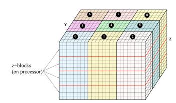
The red lines (thick gray lines) indicate computational blocks in the z direction. Each processor has Ib ×Jb×Kb cells, and each block has size Ib ×Jb×Kb cells(Evans et al., 2010).
Note: great care should be taken when defining the Denovo spatial mesh; a coarse mesh may result in unreliable importance maps, even when source biasing is implemented. The Denovo deterministic solver also utilizes a ray tracing method to generate track-length contributions (i.e., mean free path determinations) within the geometry of the problem; increasing the number of rays fired per computational domain block (mesh face) is particularly useful for large problems with small tally volumes. This is especially prevalent with the 0.5x1 and 1x1-inch detector CPM Calculator simulations.
4.2.2 CADIS Hybrid Method Overview
The hybrid capabilities of Shift are particularly useful for speeding up the transport of sources that undergo significant attenuation in large problem geometries and lowering the uncertainty associated with tally results when compared to analog (no variance reduction) MC. Shift is currently capable of neutral particle transport only for photons and neutrons and may be used to simulate select tallies that mirror those included in MCNP, such as average flux in a volumetric cell (F4 tally in MCNP). The hybrid methodology utilized in this study is known as the CADIS (Consistent Adjoint Driven Importance Sampling) hybrid method, which is a single tally region optimization method that relies on the discrete ordinates deterministic solver, Denovo, to generate an adjoint flux and associated importance map for particles simulated in a given environment. Once the adjoint flux and importance map are generated, particles are more likely to be born in regions of higher importance in the simulation environment. Omnibus code is used to couple the Denovo deterministic and Shift MC solver as part of the Exnihilo code suite to accelerate the Shift transport simulations. The CADIS hybrid method is known to be nearly 100,000 times more efficient than analog MC based on tally figure of merit (FOM) comparisons (Wagner et al., 2011).
In the CADIS method, particles are biased (increasing the number of sampled particles in order to decrease uncertainty). The biased source distribution is utilized such that particles are more likely to contribute to the total detector response and fall within the initial statistical weights (quantifies the tally contribution of particles in a simulation environment) generated from Denovo. The biased source distribution relationship is represented by the equations below (Wagner et al., 2011).


In the CADIS hybrid method, a weight window technique is applied by generating detailed space- and energy-dependent importance parameters (particle weights) and applying geometric splitting/roulette and energy splitting/roulette, while simultaneously controlling weight variations as a particle travels throughout an environment (Wagner et al., 2011). The deterministic Denovo solver generates the adjoint flux and associated weight window map; the Shift MC solver employs the stochastic splitting/roulette method in the phase space to determine the final contribution of particles in a tally region. The initial statistical weight of a particle is, w0(,r→,E), is defined by the following equation (Wagner et al., 2011).

Upon initiation of the Shift MC solver, if a particle falls below a given weight in the importance map (3-D distribution of w0(r→,E)), then the particle will be split (source biasing) or rouletted (terminated) in order to sufficiently increase its weight. This hybrid technique greatly increases the rate at which the Shift MC solver final solution converges and thus significantly increases computational efficiency.
4.3 Detector Details
Four sodium iodine (NaI) detector sizes are included in the CPM Calculator (0.5" × 1", 1" × 1", 2" × 2", 3" × 3"). Energy response curves (simulated) were created for each one using the pulse height energy deposition tally in MCNP (surface contamination) and MCNP/Shift method (volumetric contamination). The terms "pulse height", "response", and "detector response" are used interchangeably in the method to denote detector count rate. It is important to note that only the distribution of energy deposition pulses in the detector crystals are simulated; therefore, other factors that comprise the true detector response such as detector resolution, dead time, background, and pulse pile-up are unaccounted for. Nevertheless, the high-fidelity simulations of the energy deposition spectra result in conservative, yet scientifically rigorous screening value estimations of the detector count rate used to produce the GDR corresponding to a desired FAC or TAC.
The model assumes the detector is stationary and time is not considered. Any movement of the detector was not taken into account.
Schematics, images, and manufacturer instrument response curves are given below.
- Ludlum model 44-62 0.5x1 inch NaI detector
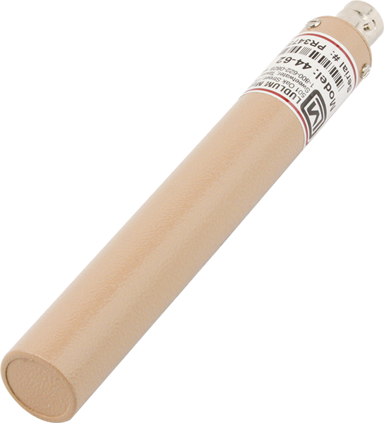
- Ludlum model 44-62 0.5x1 inch NaI detector schematic
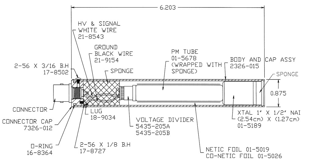
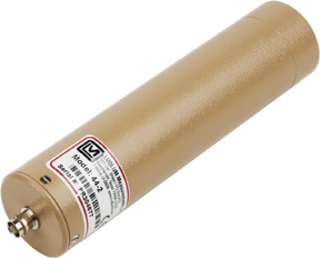
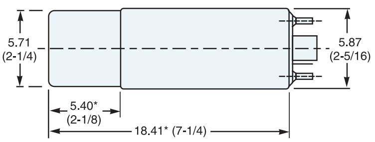
- Ludlum model 44-2 1x1 inch NaI detector
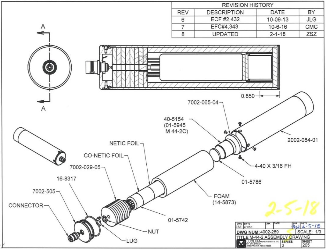
- Ludlum model 44-2 1x1 inch NaI detector schematic
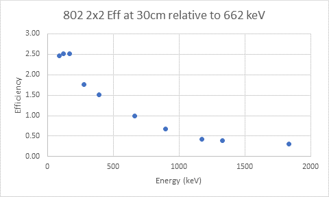
- Canberra model 802-2 2x2 inch NaI detector

- Canberra model 802-2 2x2 inch NaI detector schematic
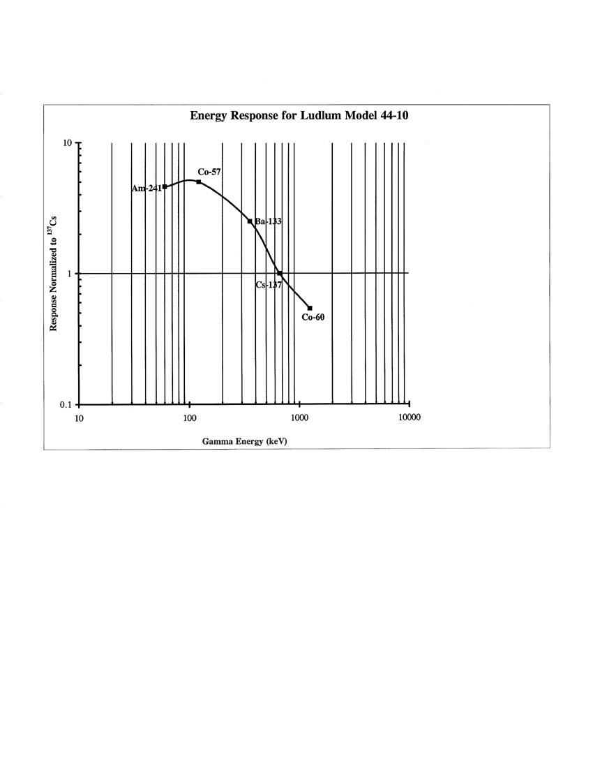
- Ludlum model 44-10 2x2 inch NaI detector
- Ludlum model 44-10 2x2 inch NaI detector schematic
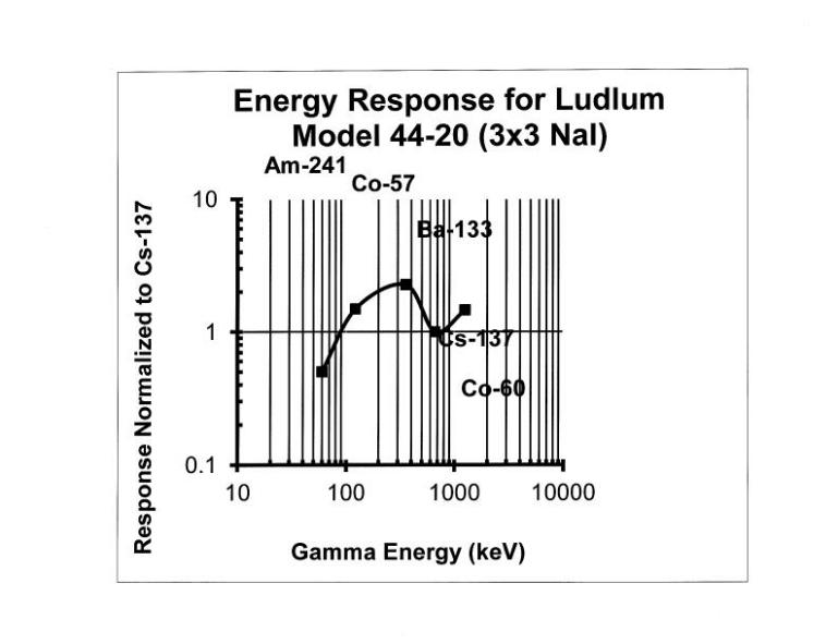
- Ludlum model 44-20 3x3 inch NaI detector
- Ludlum model 44-20 3x3 inch NaI detector schematic
4.4 Material Details
In this project, source data was obtained from a report published by Pacific Northwest National Laboratory, PIET-43741-TM-963 PNNL-15870, Rev. 1, Compendium of Material Composition Data for Radiation Transport Modeling, which is summarized in MCNP syntax in the table below (McConn et al., 2011). The exception is for the material definition of soil, which was taken from the Environmental Protection Agency's Federal Guidance Report 15 silty soil composition (Veinot et al., 2017).
Material ZAID Weight Fraction Concrete (Regular) 1,000 -0.010000 8,000 -0.532000 11000 -0.029000 13,000 -0.034000 14,000 -0.337000 20,000 -0.044000 26,000 -0.014000 Soil (FGR 15) 1,000 -0.021 6,000 -0.016 8,000 -0.577 13,000 -0.05 14,000 -0.271 19,000 -0.013 20,000 -0.041 26,000 -0.011 Steel (304 Stainless) 6,000 -0.000400 14,000 -0.005000 15,000 -0.000230 16,000 -0.000150 24,000 -0.190000 25,000 -0.010000 26,000 -0.70730 28,000 -0.092500 Drywall (Gypsum/Plaster of Paris) 1,000 -0.023416 8,000 -0.557572 16,000 -0.186215 20,000 -0.232797 Glass (Plate) 8,000 -0.459800 11,000 -0.096441 14,000 -0.336553 20,000 -0.107205 Wood (Southern Pine) 1,000 -0.059642 6,000 -0.497018 7,000 -0.004970 8,000 -0.427435 12,000 -0.001988 16,000 -0.004970 19,000 -0.001988 20,000 -0.001988 The following table presents densities, mass attenuation coefficients, and the resulting infinite four mean free path values for discrete photon emission energies (in the air above the contaminated source and surrounding the detector) to define contamination plane radius.
Energy (MeV) Mass Attenuation Coefficient µ/ρ (cm2/g) Linear Attenuation Coefficient µ (cm-1) - Mean Free Path 1/µ (cm) Plane Radius 4/µ (cm) 0.01 5.120 6.62E-03 151.05 604.22 0.02 0.778 1.01E-03 994.21 3976.84 0.03 0.354 4.57E-04 2185.97 8743.87 0.04 0.249 3.21E-04 3112.25 12449.02 0.05 0.208 2.69E-04 3718.25 14872.98 0.06 0.188 2.42E-04 4124.77 16499.10 0.07 0.177 2.29E-04 4389.09 17556.35 0.08 0.166 2.15E-04 4653.40 18613.60 0.1 0.154 1.99E-04 5018.79 20075.15 0.15 0.136 1.75E-04 5703.50 22814.02 0.2 0.123 1.59E-04 6272.47 25089.87 0.3 0.107 1.38E-04 7248.31 28993.26 0.4 0.095 1.23E-04 8099.23 32396.91 0.5 0.087 1.13E-04 8877.36 35509.42 0.6 0.081 1.04E-04 9601.43 38405.72 0.8 0.071 9.15E-05 10932.93 43731.71 1 0.064 8.22E-05 12164.13 48656.51 1.5 0.052 6.69E-05 14944.83 59779.34 2 0.044 5.75E-05 17391.39 69565.57 3 0.036 4.63E-05 21597.19 86388.74 4.5 Progeny and Chains
The CPM Calculator will consider progeny contributions to cpm following the decay method selected on its main page. The calculator offers four options that match the EPA's screening level calculators (PRG, DCC, BPRG, BDCC, SPRG, and SDCC):
- Assumes ingrowth and decay of the whole chain over time from a pure waste product without source replenishment,
- Assumes secular equilibrium throughout chain (assumes that source is continually being replenished and all progeny are at fractional activity equal to the parent and, therefore, doesn't calculate decay,
- Does not assume secular equilibrium, provides results for progeny throughout chain (calculated with decay where appropriate and the output is given for each progeny in the chain, and
- Does not assume secular equilibrium, provides results for selected isotopes only, no progeny included (calculated with decay where appropriate and the output is given for only the isotopes selected.
4.6 Model Geometry and Physics
This section describes the setup of the contaminated sources and the detector geometry in MCNP/Shift.
4.6.1 Ground Plane
The geometry of the ground plane model is a 1 micron thick disc source above which a detector is suspended. The height (h) of the detector is the user's estimate of the distance in centimeters between the detector and the source of contamination. The maximum radius of the disc (R) is calculated such that the distance from the detector to the outer circumference of the circle is four mean free paths of the simulated photon energy in air (3 MeV in the example depiction below), a distance at which the photon is safely assumed to be attenuated.
Detector responses from ground plane sources were simulated in MCNP using high-performance computing (HPC) clusters. Simulations were run for 19 monoenergetic photon sources, each using 120 combinations of contamination material, detector configuration, and source-detector distance. In each simulation, a pulse height spectrum was estimated throughout the NaI crystal of the modeled detector. All final MCNP pulse height tally results were reported with relative errors of less than 5%.
4.6.2 Volumetric
The 6 different options for source material are soil, concrete, plate glass, wood, steel, and drywall. These materials are based on a uniformly contaminated cylindrical slab source of varying thickness. The average cell flux throughout a void-filled "coupling surface" mimicking the geometry of a detector suspended in air at a distance above the source is estimated, which would be converted to average pulse height in the corresponding full model detector in a post-processing code. An example of a Volume CPM model for a 3 MeV source contaminated in soil at a discrete depth (shown in red) is depicted in this diagram.
The total depth of a medium (red and brown regions) is always based on four mean free paths for a 3 MeV source in the medium of interest.
Average cell fluxes for the Shift volumetric contamination runs were simulated using high-performance computing (HPC) clusters. All final Shift average cell flux tally results were reported with relative errors of less than 5%.
4.7 MCNP and SHIFT Implementation
The MCNP pulse-height tally may be approximated by multiplying the energy-dependent fluence (or average cell flux tally result) by a user-provided detector response function that accounts for phase space dependencies such as energy and position of photons incident on the detectors. Since the detectors of interest have dimensions that are (approximately) isotropic, an angular detector response function is not needed to account for fluctuations in the direction of photons incident on the detectors. See the following equation.

Detector response functions (RFs) were generated by normalizing the MCNP estimated pulse height for surface contamination to the average cell flux estimated using Shift for the same modeling conditions (emission energy, contamination depth, contamination material, detector configuration, and source-detector distance). See the following equation.

The detector response for monoenergetic volumetric sources was calculated as the product of the energy-binned fluence and the energy dependent response function. See the following equation.

For a given radionuclide, the detector response for each photon emission energy was interpolated from the responses of the 19 monoenergetic photon sources for the same conditions (contamination depth, contamination material, detector configuration, and source-detector distance) using the piecewise cubic hermite interpolating polynomial (PCHIP) interpolation algorithm in a post-processing code. The interpolated response at each emission energy was multiplied by the corresponding decay yield of the emitted photon, and the final radionuclide-specific response for the given conditions was calculated as the sum of the product over all emission energies. It was assumed that photons with emission energies below 20 keV did not contribute to the final response and were, therefore, omitted from the calculation.
4.8 Calculating the Activity Concentration to CPM Conversion Factor
4.8.1 Ground Plane Source Contamination
The MCNP pulse heights were normalized, as presented in the equation below, to obtain the ith monoenergetic or radionuclide ground plane source activity concentration to CPM conversion factor.

4.8.2 Volumetric Source Contamination
The MCNP/Shift responses (MCNP-equivalent pulse heights) were normalized, as presented in the equation below, to obtain the ith monoenergetic or radionuclide volumetric source activity concentration to CPM conversion factor.

4.9 Converting the Field and Target Activity to CPM
Field Activity Concentration in CPM, cpmFAC, and Target Activity Concentration in CPM, cpmTAC, are found by multiplying the cpm per activity concentration conversion factor, CF, by the user's TAC in pCi/g for a radionuclide. If multiple primary radionuclides were selected, the FACs in pCi/g are also multiplied by the result. The equations for cpmFACi and cpmTACi for a radionuclide i may be seen below.


4.10 Calculating the Relative Fraction
The relative fraction, f, is the fraction of the total activity contributed by each radionuclide. The FACs are used to find the relative fractions of each radionuclide, which are then applied to the GDR. The equation for calculating the relative fraction for a radionuclide i may be seen below.

4.11 Calculating the Gross Detector Response
The GDR is the total calculated response of the detector in cpm for the desired remedial activity of the particular radionuclides in the soil. MARSSIM Equation 4-4 "Gross Activity DCGL" (U.S. EPA, 2000) is applied to find the GDR and can be seen in an edited form below.

where f is the relative fraction of each radionuclide and cpmTAC is the TAC of each radionuclide in units of detector cpm.
5. Definitions of Terms and Acronyms
Table 1 presents the definitions of the variables and their default values.
Table 1. Definitions of Terms and Acronyms
| Symbol | Definition (units) | Default | Reference |
| CFi | CPM conversion factor (cpm/(pCi/cm2) or cpm/(pCi/g)) | Isotope-specific | Calculated TAMU 2020 |
| GDR | Gross detector response (cpm) | Isotope-specific | Calculated |
| FAC | CPM conversion factor (cpm/(pCi/cm2) or cpm/(pCi/g)) | Isotope-specific | Calculated |
| TAC | CPM conversion factor (cpm/(pCi/cm2) or cpm/(pCi/g)) | Isotope-specific | Calculated |
| f1 | Relative fraction (unitless) | Isotope-specific | Calculated |
6. References
Asano, E., Coleman, D., Davidson, G., Dewji, S. 2022. Photon Detector Response Function Methodology Using MCNP and Shift Hybrid Radiation Transport Code for Wide-Area Contamination Assay Applications. Nuclear Instruments and Methods in Physics Research Section A: Accelerators, Spectrometers, Detectors and Associated Equipment, 1031, 166568. May 11, 2022. Available at: https://www.sciencedirect.com/science/article/abs/pii/S0168900222001668.
Bellamy, M., Eckerman, K., Fillingame, B., Dolislager, F. 2013. Monte Carlo Calculation of Photon Flux to Support the EPA CPM Volume Calculator. Oak Ridge National Lab, Oak Ridge, TN 37831. Available here.
Berger, M., Hubbell, J., Seltzer, S., Chang, J., Coursey, J., Sukumar, R., Zucker, D., Olsen, K. 2010. XCOM: Photon cross sections database, NIST Standard Reference Database 8 (XGAM) [Online]. Available at: https://www.nist.gov/pml/xcom-photon-cross-sections-database. [Accessed 2020].
Biondo, E.D., and Wilson, P.P.H. 2017. Fusion energy systems analysis with the groupwise transmutation CADIS method. International Conference on Mathematics and Computational Methods Applied to Nuclear Science and Engineering. Available at: https://inis.iaea.org/search/search.aspx?orig_q=RN:53074336.
Evans, T.M., Stafford, A.S., Slaybaught, R.N., Clarno, K.T. 2010. Denovo: A New Three-Dimensional Parallel Discrete Ordinates Code in SCALE. Nuclear Technology, 171:2, 171-200, DOI: 10.13182/NT171-171.
Hubbell, J. & Seltzer, S. 1996. X-Ray Mass Attenuation Coefficients [Online]. Available at: https://www.nist.gov/pml/x-ray-mass-attenuation-coefficients. [Accessed 2020].
ICRP. 2008. Nuclear Decay Data for Dosimetric Calculations. Ann. ICRP), 38(3). Available at: https://www.icrp.org/publication.asp?id=ICRP%20Publication%20107.
Los Alamos National Laboratory (LANL). 2003. MCNP - A General Monte Carlo N-Particle Transport Code, Version 5, Volume I: Overview and Theory. X-5 Monte Carlo Team, LA-UR-03-1987. April 24, 2003 (revised February 2008).
Ludlum Measurements Inc. (Mcconn, R.J., Gesh, C.J., Pagh, R.T., Rucker, R.A., Williams III, R.). 2011. Compendium of material composition data for radiation transport modeling. Pacific Northwest National Lab (PNNL), Richland, WA (United States). Available at: https://ludlums.com/products/all-products/category/gamma-scintillator.
McConn Jr., R.J., Gesh, C.J, Pagh, R.T., Rucker, R.A., Williams III, R.G. 2011. Compendium of Material Composition Data for Radiation Transport Modeling. PNNL, PIET-43741-TM-963, PNNL-15870, Rev. 1. Available at: https://www.pnnl.gov/main/publications/external/technical_reports/PNNL-15870Rev1.pdf.
Mirion Technologies. 2022 (accessed). Model 802 Scintillation Detectors. Avaialable at: https://www.mirion.com/products/802-scintillation-detectors.
Pandaya, T.M., Johnson, S.R., Evans, T.M., Davidson, G.G., Hamilton, S.P., Godfrey, A.H. 2016. Implementation, Capabilities, and Benchmarking of Shift, A Massively Parallel Monte Carlo Radiation Transport Code. Journal of Computational Physics, 308, 239-272. March 1, 2016. Availabe at: https://www.sciencedirect.com/science/article/pii/S0021999115008566.
Schwarz, A.L., Schwarz, R.A., Carter, L.L. 2011. MCNP/MCNPX Visual Editor Computer Code.
Texas A&M University (TAMU). 2020. Final Report for project entitled CPM Modeling. December 2020. Availabe here.
U.S. Environmental Protection Agency (EPA). 2000. Multi-Agency Radiation Survey and Site Investigation Manual (MARSSIM). NUREG-1575, Rev. 1; EPA 404-R-97-016, Rev. 1; DOE/EH-0624, Rev. 1. Available at: https://www.epa.gov/sites/default/files/2017-09/documents/marssim_manual_rev1.pdf.
Veinot, K.G., Eckerman, K.F., Bellamy, M.B., Hiller, M.M., Dewji, S.A., Easterly, C.E., Hertel, N.E., Manger, R. 2017. Effective dose rate coefficients for exposure to contaminated soil. Radiat Environ Biophys, 56(3), 255-267.
Wagener, J.C., Peplow, D.E., Mosher, S.W., Evans, T.M.. 2011. Review of Hybrid (Deterministic/Monte Carlo) Radiation Transport Methods, Codes, and Applications at Oak Ridge National Laboratory. Progress in Nuclear Science and Technology, 2, 808-814.
Werner, C.J. (ed.). 2017. MCNP user's manual - code version 6.2. Available at: MCNP User's Manual. [Accessed 2020].